The art of cabling

The challenge of organising your cables behind your TV is nothing compared to that of a large computing cluster.

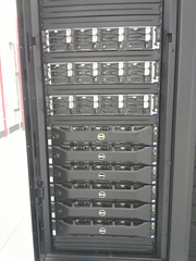
One of our standard racks contains 12 Dell R510s servers (for storage) and 6 Dell C6100 chases (providing 24 compute nodes) all 36 nodes are connected with a 10 Gb (SFP+), 1 Gb (backup) and 100 Mb (for IPMI) network cable. Connecting to 3 different network switches at the top of the rack. In addition the 18 "boxes" need a total of 36 power connections. A total of 144 cables per rack!

How to cope? Separate the network cables from the power cables, a possible source of noise. Use different colour cables for the different traffic and add unique id number for each cable. Use lose, removable cable ties. When a cable brakes don't remove it, just add a new cable.

The 10 Gb switches, in our case Dell S4810s, connect using 4 40Gb QSFP+ cables to two Dell Z9000 core switches. Having two core switches allows us to take one unit out of service without downtime (we use the VLT protocol and it works!). However this does add cable complexity. The backup 1 gig switches connect to each other in a daisy chain using 10 Gb cx4 cables, left over from before our 10 Gb upgrade. Finally the ipmi switches connect to a front-end switch using 1GBaseT cables.

The picture shows the inter-switch links. Visible are the orange 40Gb connections and blue 10Gb cx4 cables. In addition each 40 Gb cable has an ID indicating which rack it came from and which core switch its going too.

We have one rack full of critical, world facing servers. These servers need to be available all the times making it very difficult to reorganise the cabling. As a result over time, as we add and remove servers, the cabling becomes a mess. This is starting to become a risk! We are just going to have to accept some down time to sort it out in the near future.

virtualization performance hit

Like the rest of the world,  there is a lot of discussion going about the use of clouds and virtualization in gridpp. 

http://www.gridpp.ac.uk/gridpp30/mcnab-lhcb-vmclouds-march-2013.pdf

http://www.admin-magazine.com/HPC/articles/the_cloud_s_role_in_hpc

Using virtualization will have a performance impact, so using it for our type of computing (hpc/htc) may not be the best solution. However just what impact does it have? A quick search of the web suggests anywhere between 3 to 30%. Most of the overhead appears to be in the kernel and in i/o.

http://serverfault.com/questions/261974/how-much-overhead-does-x86-x64-virtualization-have

http://www.altechnative.net/2012/08/04/virtual-performance-part-1-vmware/

http://www.anandtech.com/show/3827/virtualization-ask-the-experts-1

I decided that I wanted to do some of my own tests with the focus on the type of work we do in gridpp. 

Testbed: 24 thread westmere processor running at 2.66 GHz + 48 Gig of memory using Scientific Linux 6.3 (basically RHEL6). I'm using the default install of KVM with the virtual image as a local file setup to use all 24 threads.

Benchmarks: 1) I unpack and make the ROOT analysis package using 24 threads; 2) as 1 but using only one thread. 3) I generate 500,000 Montecarlo events using the HERWIG++ Generator; 4) as 3 but I also include the time taken to unpack and install HERWIG++; 5) I run the HEP-SPEC06 benchmark. For tests 1 to 4 i use the TIME command to obtain the real time taken (smaller is better), for 5 I report the hep-spec score (larger is better).  I will run the benchmarks on the bare metal install and on the VM on the same hardware and compare the results.

Results:

Out of the box performance of KVM results in ~3% (CPU intensive) to 20% (sys call intensive) reduction in performance. There is some indication of correlation with ratio of sys time / user time (particular effect with make/tar/gzip?). This is not seen in HEP-SPEC result. SYS time is the CPU time spent within the kernel and from previous studies we expect this to incur a high performance hit in virtualization.

If I get the time I intend to repeat analysis using optimisations (e.g. guest image on LVM). Repeat analysis using fedora 18 ( ~RHEL 7). Repeat using sandybridge cpu. Look at network performance (eg iozone with lustre).

The Queen Mary Grid Cluster

The qmul grid/htc cluster is a high throughput (htc) research computing cluster based at Queen Mary, University of London. We primarily serve the scientific grid community and are funded by the griddpp
collaboration (i.e. uk stfc research council). By high throughput we mean the ability to do lots of individual separate jobs. Our main workload is data analysis for the ATLAS experiment at cern. We are the top site in the UK for this type of work, and one of the leading sites for the ATLAS LHC experiment in the world. We are part of the LondonGrid (hence the post to this blog!)

Our cluster comprises of:

For running the actual jobs
30 Dell C6100 using X5650s processors, contributing a total of 2880 job slots, and
60 older streamline nodes using E5420 processors, contributing a total of 480 job slots.

For Storage we run the Lustre parallel file system using
72 Dell R510s with 1800 TBytes of disk and
12 older Dell 1950s with MD100 disk arrays with 360TB of disk
Our actual provision is about 1600TB due to the use of raid 6 and "real" disk sizes.

We have a lot of development work to do over the next year which I hope to describe over the coming month in this blog including...

• A new monitoring system probably based on opennms.
• A new deployment system, to replace our hand made perl/mason/kickstart system probably using razor and puppet.
• A cloud stack, we've been doing scientific computing using the grid software, but this model of computing is likely to be replaced with a cloud type model, we will need to look at the various options (OpenStack, CloudStack or OpenNebula).

The 11 racks of the QMUL cluster

RHUL cluster expands

Yesterday, RHUL took delivery of new storage and compute nodes to beef up its Tier2 cluster.
The GridPP and CIF funded kit was supplied by Dell and is being installed and configured by Alces.
The extra 6.3 kHS06 and 420 TB will more than double the capacity of cluster.
Once the installation is complete and accepted, work to integrate it with the existing cluster and bring up the gLite services will begin.

RHUL 'Newton' cluster comes home

After two years hosted by Imperial College, our 'Newton' Grid computing cluster has finally been relocated to Royal Holloway's new state-of-the-art computer centre. The move was carried out by Clustervision and everything went smoothly. Before the cluster goes back into production, analysing LHC data, a software upgrade to SL5 is planned.

A small part of Newton remains at IC: the racks were donated to become part of the particle physics cluster.

Comparing ATLAS analysis at RHUL using the file-staging and RFIO approaches

I have been looking at the performance of the Royal Holloway cluster during Hammercloud tests in which data was accessed directly from the DPM pool nodes using the RFIO protocol and comparing it to the recent UK-wide file-staging test (540).

For the RFIO approach two identical tests (537 and 538) were requested in order to ensure enough jobs arrived on site. The RFIO IOBUFSIZE was set to 4KB. Job CPU efficiencies and cluster throughput (the product of number of running jobs and average job efficiency) were extracted using Sam and Dug's script. The job throughput climbed steadily up to a peak at around 320 running jobs. At this point the throughput started to decline probably compounded by the fact that one of the disk servers lost a disk and became over-loaded.


The CPU efficiency declined relatively consistently as the number of running jobs increased:


Each job was reading data at about 1 MB/s so that at the peak the total bandwidth was around 350 MB/s - roughly 30 MB/s per disk server. The disk servers were working hard, however, the iostat %util values were around 100% with high cpu iowait values.

So how do these results compare to those obtained when staging files to the worker node prior to analysis? This graph shows the same RFIO throughput data together with results from the recently run file-staging test:



The throughput during file-staging leveled off earlier - at around 175 running jobs. Similarly the average job efficiency drops more steeply:


The job failure rate for the RFIO tests was 4% compared to 17% for the file-staging test.

RHUL getting good rates into MCDISK from RAL

RHUL has regularly got good rates and by that I mean 80-100 MB/s from Fermilab when downloading CMS data. It nice now to see similarly high rates downloading ATLAS data into the MCDISK space token from RAL.